Doing some biological modeling

At my new job our focus is to uncover scientific insights to accelerate and improve scientific research. I’m a data engineer by trade, but the science side of the business bleeds in to what I do on a fairly regular basis. Without the scientific and research background that many of my peers have, I feel the need to do some self improvement in those areas. So I was happy to find a series of videos on youtube titled Computational Biology with Python (Modeling Gene Networks) created by Mike Saint Antoine

The video series centers around modeling ordinary differential equations and stochastic differential equations using python, specifically for gene expression, and the central dogma of molecular biology. This was great for me, because that is a topic that has come up at work, so it was a great chance to bridge my history of working with code, and my ancient (university days) history of working with math.

The central dogma of molecular biology is that information flows from DNA to mRNA to proteins. That is DNA is transcibed into mRNA and mRNA expresses proteins. I think.

DNA ➡ mRNA ➡ protein

This is modeled roughly as:

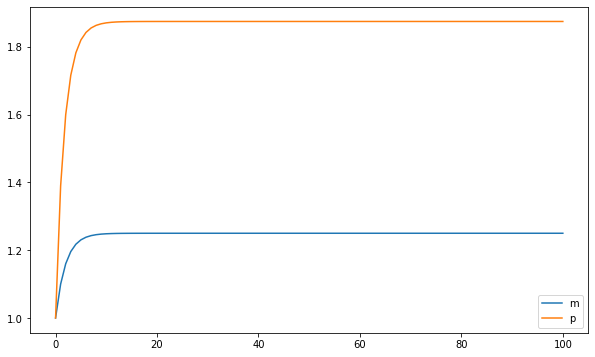
mrna_change = k_m - gamma_m * m
protein_change = k_p * m - gamma_p * p

So the amount of mRNA has a constant upward change, but it slows down as more mRNA is present. And the amount of the protein goes up proportional to the amount of mRNA present and decreases proportional to the amount of protein present.

I went ahead and coded the model for myself before the videos showed a solution. Here’s my code:

m_0 = 1.0
p_0 = 1.0
gamma_m = 0.4
gamma_p = 0.6
k_m = 0.5
k_p = 0.9

def next_m_p(m, p):
    m += k_m - gamma_m * m
    p += k_p * m - gamma_p * p
    return (m, p)

m = m_0
p = p_0
mps = [(m, p)]
for _ in range(100):
    m, p = next_m_p(m, p)
    mps.append((m, p))

This gives a plot like this, which the next video showed how to do with odeint:

The course goes on to talk about more complex systems and finishes with a stochastic model of a 3 gene oscillating system with I think was called a Goodwin Oscillator.

Way back in my university days I took a course in fourth year called Mathematical Modeling, with professor Kenzu Abdella. In those days I did almost all of my coding in Maple, which is basically Canada’s mathematica. I haven’t used it in 15 years or so, but I’d say it’s a functional language used mostly for symbolic manipulation and equation solving. I spent many late nights working in maple trying to do my year-end project for that course.

I was trying to replicate and hopefully improve the Lotka-Volterra predator prey population model. The idea of the model is that predator and prey population levels are dependent. An over-population of prey leads to higher levels of predators, which leads to a population crash in prey, then the predator population crashes. So both are cyclical, but there is a lag between the cycles. Honestly I remember that finding a data set of predator and prey populations was more challenging than the math or coding aspect. And I’ve found that finding good data is often the hardest part in a modelling exercise.

Because of my experience with this model, I decided to try my hand with knowledge from the video series on the Lotka- Volterra model with the techniques from the video.

First, here’s how I would do it before having watched the videos:

# started with the values from wikipedia for these
# then fiddled until I got something reasonable.
alpha = 0.0075
beta = 0.133
delta = 0.10
gamma = 0.10
x0 = 0.5
y0 = 0.1

def next_xy(x, y):
    return (x + alpha * x - beta * x * y, 
        y + delta * x * y - gamma * y)

Which gives this:

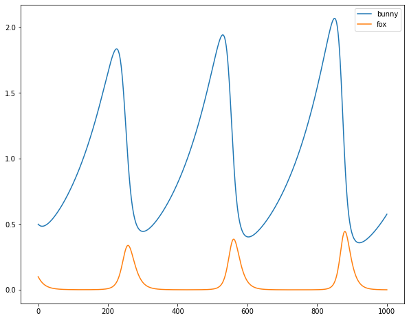
I’m not a population biologist or whatever, but I think this looks pretty nice.

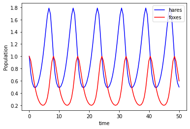
And here’s how the problem would be solved using the technique from the videos:

def sim(variables, t, params):
    x, y = variables
    alpha, beta, delta, gamma = params
    dxdt = alpha * x - beta * x * y
    dydt = delta * x * y - gamma * y

    return([dxdt, dydt])
# I think the wikipedia values worked here.
alpha = 0.66
beta = 1.33
delta = 1.0
gamma = 1.0
params = (alpha, beta, delta, gamma)
t = np.linspace(0, 50, num=100)
y0 = [1,1]

y = odeint(sim, y0, t, args=(params,))

Which gives this plot:

I tried to do the stochastic model but I couldn’t get it working. I noticed that Mike Saint Antoine has a couple videos about Lotka-Volterra, so I’ll probably check those out at a later date and see what I was doing wrong.