Bayes’ theorem is a way of determining the likelihood of an event A given that another event B has occurred. It’s a way of making an educated guess without much information to go on.

It’s a way of going from knowing the likelihood of evidence, given a known outcome to knowing the likelihood of a known outcome given existing evidence. E.g. What’s the likelihood tacos are for dinner? If we know the likelihood of tacos, the likelihood of a meal being dinner, and the likelihood of tacos, given that it’s dinner, we can find this out.

Bayes’ Theorem gives you an idea of how much you should trust the evidence you have. If your evidence is weak, you won’t end up trusting it. For example, I’m sure my neighbours don’t think that our house is on fire every time they hear my fire alarm going off at supper time. (But it is pretty good evidence that I’m a lousy cook.) They’ve lost their trust in the evidence that my fire alarm gives that our house is on fire.

Say you are looking for P(A|B), the probability of event A occurring given the fact that we have the evidence B. For this to work, you need to know:

P(B|A): The probability that an event B is an A
P(A): The probability of A occurring. (This is often called the prior probability of A.)
P(B): The probability of B occurring.

Given these data, you can put the numbers into the following equation:

P(A|B) = P(B|A) * P(A) / P(B)

You might ask: “How do we get this equation?” We can start with the axiom of probability: P(A and B) = P(A given B)P(B). This axiom is saying that the probability of two things happening is the same as the probability that one thing happened, given that the other already happened.

This gets us 90% of the way to Bayes’ Theorem. From the axiom, you see that P(A given B) = P(A and B)/P(B). Now use P(B and A) = P(A and B), and reverse the terms in the axiom to get P(A given B) = P(B given A)P(B)/P(A).

A Simple Example

Suppose you have two bags containing marbles. Bag A contains 2 red balls and 1 yellow ball. Bag B contains 1 red ball and two yellow balls.

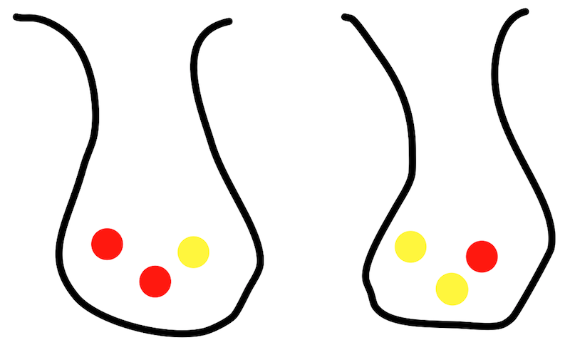
You don’t know which bag is which.

If you pull a yellow ball of a bag, what is the probability that it is bag A? We have an intuitive feeling that it’s most likely Bag B, but Bayes’ can give us an exact answer. This will be given by:

P(Bag A given a yellow ball being pulled) = P(Yellow ball given bag A) * P(bag A) / P(yellow ball)

P(yellow ball given bag A)``: This is the number of yellow balls (1) in bag A divided by the total number of balls in bag A (3), so1/3`.
P(bag A): This is the number of bags that are bag B (1) divided by the number of bags, so ‘1/2’.
P(yellow ball): This is the probability of drawing a yellow ball from any bag. Thus it’s the total number of yellow balls across all bags (3), divided by the total number of balls in all bags (6), so ‘3/6’

Plugging these values in, we get the following:

P(Bag A|yellow) = (1/3) * (1/2) / (3/6)

The result is 1/3. So we know that if we reach our hand into one of bag A and bag B, and draw a yellow ball, that the probability that we reached into bag A was 1/3. This matches our intuition, but Bayes’ Theorem is most well known for it’s intuition defying examples.

A mind-expanding example

You’re walking down the hall at work. You see someone walk out of the software development wing who is odd. You wonder to yourself: is this person a Fortan developer? Your sneaking suspicion is that this odd person is probably a Fortran developer because you have a feeling like Fortran developers are mostly odd. Let’s work through an example.

P(fortran developer, given odd) = P(odd, given Fortran developer) * P(fortran developer) / P(odd)

Let’s substitute in some estimates for these values.

P(odd, given fortran developer): Let’s say 85% of fortran developers are odd.
P(fortran developer): Most developers are average and use react. Only 1% of all developers use Fortran.
P(odd): Across the whole company, you estimate that 10% of developers are odd.

Let’s plug the numbers into Bayes’ theorem and find out whether the odd person we have observed is probably a Fortran developer:

P(fortran developer, given odd) = (0.85) * (0.01) / (0.1)

And the answer is 0.085, or 8.5%. This runs counter to the original intuition that the developer must be a fortran developer because they are odd. While it’s true that most fortran developers are odd, there are so few fortran developers total, meaning that most of the time an odd developer is not a fortran dev.

The odd Fortran developers are outnumbered by the comparatively less common odd react developers, but that the total number of odd react developers is still higher. So just because someone is odd, it doesn’t make them a Fortran developer.

Learning Through Bayes’ Theorem

This is all super interesting and cool, but there’s an even more cooler application of this theory we can look at. Notice how the prior probabilities we worked with in the examples before were static. We can continually update these to get a better model of our simulation as we encounter new data. Assuming that the model behaves consistently, we will get continually better results.

A historical example of this line of reasoning comes from a thought experiment performed by Thomas Bayes. The experimenter asks an assistant to throw a ball onto a table (for the sake of the experiment, it doesn’t bounce or roll). The goal of the experiment is to determine the location of this ball without being able to see its location. The assistant would then throw ball after ball onto the table and tell the experimenter whether each successive ball landed to the left or right, and behind or in front of the first ball. By running successive trials, the experimenter can update their view of where the ball might be. For example, if most subsequent balls are reported as being to the left of the first ball, it’s safe to guess it’s near the right side of the table. Bayes’ Theorem lets us quantify this measurement.

A proper learning example

Now we’ve seen how we can apply a learning and Bayes’ to improve our predictions using probability. Let’s apply the same to classifying something a bit more complex. Here we will be tracking multiple probabilities and combining those to predict a classification of a document.

This technique assumes that we have a training set of data where a human has manually gone through and confirmed the classifications of a group of documents.

Example of headlines and news category:

text

classification

Local Team Loses Game

sports

Player Loses Game

sports

Movie breaks box office record

entertainment

English team scores goal

sports

gravity waves recorded using machine

science

New Comedy Is A Good Movie

entertainment

New Global Warming Movie

science

…

Using this data we can train a classifier… Let’s break down the results by word and see which words tend to be in certain categories:

word

P(sports)

P(entertainment)

P(science)

Local

1 / 1

Team

2 / 2

Loses

2 / 2

Game

2 / 2

Player

1 / 1

Movie

2 / 3

1 / 3

breaks

1 / 1

box

1 / 1

office

1 / 1

record

1 / 2

English

1 / 1

Scores

1 / 1

Goal

1 / 1

Gravity

1 / 1

Waves

1 / 1

Using

1 / 1

Machine

1 / 1

New

1 / 2

Comedy

1 / 1

Good

1 / 1

(Note that this data will work for an example, but for good results you would want a much larger training set than this.)

Here we can see the prior probabilities of a given word in a title affecting the classification of the document. Now let’s assume that we fed millions of headlines into this system and ended up with something like this:

word

P(sports)

P(entertainment)

P(science)

Local

33000

Team

35578

Loses

29666

200

…

And so on. This gives an example of how sports-centric terms will train to give high probabilities of related documents landing in the sports category. The prior evidence here is strong.

When we want to classify a new document, how do we compute the probability of it being in a given class, now that it has multiple terms? First, let’s think about what it would mean if there were only two terms to worry about.

P(sports, given win AND team) = P(win, given sports AND team) * P(team given sports) * P(sports) / (P(win AND team) * P(team))

This is already complex for only two terms, but let’s look at a simpler way to look at this. We can assume independence of the terms. This may not be the most accurate model but it will give us results that we can work with and evaluate. This assumption that the terms are independent makes calculation simple, but it’s also not entirely accurate, hence why this technique is called ‘naive’. This is the ‘bag of words’ technique commonly used in NLP. For example, headlines that contain ‘delicious’ would tend to occur more often with ‘cake’ than ‘manure’, meaning ‘delicious’ and ‘cake’ have a dependence. Naive Bayes’ classifiers can compete very well against other classifiers in terms of accuracy, but we need to be mindful of this limitation that we have imposed on ourselves.

If we assume that instances of ‘win’ and ‘team’ in a sentence are independent, (which they aren’t entirely), we get an easier formula where we already have the answers in our table.

P(sports, given win AND team) = P(win given sports) * P(team given sports) * P(sports) / (P(win) * P(team))

This will be a lot easier to calculate. And we can generalize this formula:

P(sports, given words) = (product of each P(word|sports)) * P(sports) / (product of each P(word))

With this formula in hand, we just have to iterate through each classification to determine if a document is in a given class, then we can report the most likely classification along with it’s probability. If a user confirms the classification, then we can add the new information to the prior probability table.

So how would you implement this?

Generally as a developer it’s best to reach for a pre-built tool rather than making your own. You don’t usually make yourself a hammer every time you see a loose nail. Similarly it’s best to reach for a pre-built library that can handle this kind of classification for you.

But there is real value in understanding how algorithms work. So let’s take a look at how one would implement a naive Bayesian classifier.

What would the psuedo-code look like?

classify classes = [], document:
  max_class, max_score = null, 0
  for (class : classes) {
    score = get_score(class, d)
    if score > max_score
      max_class = class
      max_score = score
  }
  return max_class;

get_score class, document:
  score = log(get_prior(class))
  features = tokenize(doc)
  for(feature : features) {
    score += log(getProbability(feature))
  }
  return score;

Here we have two methods. classify is pretty self explanatory. It’s just finding the maximum scored class for the given document. get_score is more interesting. Here is where we apply naive Bayes to calculate the scores for each class. Notice two things:

We’re using log and addition instead of multiplication. This is typical in NB implementations. This is done to avoid issues with underflow in floating point numbers. But the result is the same; adding logs is equivalent to multiplication (just ask your slide rule). But this log arithmetic means that the number we’re getting here isn’t a probability. That’s fine because we just want to find with class gives the highest number.
Notice how we don’t divide by the denominator P(B), this is because it’s a constant across all of our documents so there is no need to repeatedly do this calculation since we’re just looking for a the highest number, not a probability.

An important part is missing here, we didn’t compute the tables of prior probabilities. As mentioned before, we can do that by working through a collection of pre-classified training documents and building up counts of which features lead to which classes. Let’s look at how that might look:

train class, features:
  increment_class(class)
  for (feature : features) {
    increment_feature(feature, class)
  }

The training will keep track of the occurrence of the different class and the occurrence of different features within each class.

Here is a working example in old-fashioned javascript that does the same thing:

function Bayes() {
  this.features = {}
  this.categories = {}
}

Bayes.prototype.getScore = function(category, features) {
  score = Math.log(this.getPrior(category))

  for(var feature of features) {
    score += Math.log(this.getProbability(feature, category))
  }

  return score
}

Bayes.prototype.getPrior = function(category) {
  return (this.categories[category] || 0.1) / this.totalDocuments
}

Bayes.prototype.getProbability = function(feature, category) {
  return (this.features[category][feature] || 0.1) / this.categories[category]
}

Bayes.prototype.classify = function(features) {
  let maxClass = null
  let maxScore = -Infinity
  for (var category in this.categories) {
    const score = this.getScore(category, features)
    if (score > maxScore) {
      maxClass = category
      maxScore = score
    }
  }
  return maxClass
}

Bayes.prototype.incrementTotal = function(category) {
  this.totalDocuments = (this.totalDocuments || 0) + 1
}

Bayes.prototype.incrementCategory = function(category) {
  this.categories[category] = (this.categories[category] || 0) + 1
}

Bayes.prototype.incrementFeature = function(feature, category) {
  if (!this.features[category]) {
    this.features[category] = {}
  }
  this.features[category][feature] = (this.features[category][feature] || 0) + 1
}

Bayes.prototype.train = function(category, features) {
  this.incrementTotal()
  this.incrementCategory(category)
  for (var feature of features) {
    this.incrementFeature(feature, category)
  }
}

b = new Bayes()

b.train('city', ['subway', 'tower', 'hotel'])
b.train('city', ['opera', 'tower', 'hotel'])
b.train('city', ['opera', 'subway', 'hotel'])

b.train('country', ['cow', 'field', 'hill'])
b.train('country', ['cow', 'field', 'farm'])

// city
console.log(b.classify(['subway', 'hill', 'tower']))

// country
console.log(b.classify(['farm', 'hill', 'sheep']))

And that is it. We’ve successfully used Bayes’ Theorem to classify documents.

Intro to Bayesian Classifiers

A Simple Example

A mind-expanding example

Learning Through Bayes’ Theorem

A proper learning example

So how would you implement this?

references